Related Resources: calculators
Flat Belt Drive Design Calculator and Equations
Flat Belt Design Engineering Data
Flat Belt Drive Design Calculator and Equations
Flat belts have high strength, can be used for large speed ratios (>8:1), have a low pulley cost, produce low noise levels, and are good at absorbing torsional vibration. The belts are typically made from multiple plies, with each layer serving a special purpose. A typical three-ply belt consists of a friction ply made from synthetic rubber, polyurethane, or chrome leather, a tension ply made from polyamide strips or polyester cord, and an outer skin made from polyamide fabric, chrome leather, or an elastomer. The corresponding pulleys are made from cast iron or polymer materials and are relatively smooth to limit wear. The driving force is limited by the friction between the belt and the pulley. Applications include manufacturing tools, saw mills, textile machinery, food processing machines, multiple spindle drives, pumps, and compressors.
Preview Flat Belt Drive Design Calculator
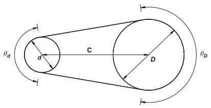
Figure 1, Belt drive geometry definition
For the simple belt drive configuration shown in Figure 1, the angles of contact between the belt and the pulleys are given by
Eq. 1
Eq. 2
where
d = diameter of the small pulley (m),
D = diameter of the large pulley (m),
C = distance between the pulley centers (m),
θd = angle of contact between the belt and the small pulley (rad),
θD = angle of contact between the belt and the large pulley (rad).
The length of the belt can be obtained by summing the arc lengths of contact and the spanned distances and is given by
Eq. 3
The power transmitted by a belt drive is given by
Eq. 4
P = ( F1- F2 ) ·V
where
P = power (watts)
F1 = belt tension in the tight side (N),
F2 = belt tension in the slack side (N),
V = belt speed (per ms).
The torque is given by
Eq. 5
T = ( F1- F2 ) · r
Assuming that the friction is uniform throughout the arc of contact and ignoring centrifugal effects, the ratio of the tensions in the belts can be modeled by Eytlewein's formula
Eq. 6
where
µ = coefficient of friction,
θ = angle of contact (rad), usually taken as the angle for the smaller pulley.
The centrifugal forces acting on the belt along the arcs of contact reduce the surface pressure. The centrifugal force is given by
Eq. 7
where
ρ = density of the belt material (kg/m3),
A = cross-sectional area of the belt (m2),
m = mass per unit length of the belt (kg/m).
The centrifugal force acts on both the tight and the slack sides of the belt, and Eytlewein’s formula can be modified to model the effect:
Eq. 7a
eµθ = (F1 - Fc ) / ( F2 - Fc )
The maximum allowable tension, F1,max, in the tight side of a belt depends in the allowable stress of the belt material, smax. Typical values for the maximum permissible stress are given in Table 1
Eq. 8
F1,max = σmax · A
The required cross-sectional area for a belt drive can be found from
Eq. 9
where
σ1 = stress belt tight side, M·N/m2
σ2 = stress belt slack side, M·N/m2
Typical values for the maximum permissible stress for high-performance flat belts.
Multiply structure |
Maximum permissible stress (MN/m2) |
||
Friction surface coating |
Core |
Top surface |
|
Elastomer |
Polyamide sheet |
Polyamide fabric |
8.3 -19.3 |
Elastomer |
Polyamide sheet |
Elastomer |
6.6-13.7 |
Chrome leather |
Polyamide sheet |
None |
6.3-11.4 |
Chrome leather |
Polyamide sheet |
Polyamide fabric |
5.7-14.7 |
Chrome leather |
Polyamide sheet |
Chrome leather |
4-8 |
Elastomer |
Polyester cord |
Elastomer |
Up to 21.8 |
Chrome leather |
Polyester cord |
Polyamide fabric |
5.2-12 |
Chrome leather |
Polyester cord |
Chrome leather |
3.1-8 |
Mechanical Design Engineering Handbook
Peter R. N. Childs
2014
Related:
- V&Flat Belt Design Equations and Formulae
- Flat Belt Design Equations
- Flat Belt Length and Pulley Center Distance Calculation
- Flat Belt Length Distance Calculator
- Motor Shaft Load Due to Belt Loading Equations and Calculator
- V Belt Application and Design Considerations
- Tension Relation of Flat Belt
- Design Horsepower Vs Service Factor
- Torque Transmitted by Belt Equation
- Rated Power of a Belt
- Tension Relation of Flat Belt
- Flat Belt Length and Pulley Center Distance Calculation
- Large and Small Diameter Lifting Pulley / Drum Equation and Calculator
- Two Lifting Lifting Pulley's Mechanical Advantage
- Synchronous Timing Belt Pulley Mechanical Tolerances per. ANSI RMA IP-24
- Synchronous Timing Belt Standard Widths and Tolerances per. ANSI RMA IP-24
- Synchronous Timing Belt Pulley and Flange Dimensions Table per ANSI / RMA IP-24
- Synchronous Timing Belt Tooth Section Dimensions Table per ANSI / RMA IP-24
- Synchronous Timing Belt Standard Pitch Lengths and Tolerances per. ANSI RMA IP-24 Table
- Synchronous Timing Belt Torque Rating Equation and Calculator per. ANSI RMA IP-24 for small pitch MXL section belts
Link to this Webpage:
© Copyright 2000 -
2024, by Engineers Edge, LLC
www.engineersedge.com
All rights reserved
Disclaimer |
Feedback
Advertising
| Contact