Finite Element Analysis FEA Review
Engineering Analysis and Design Menu
The Finite Element Analysis (FEA) is a numerical method for solving problems of engineering and mathematical physics. Useful for problems with complicated geometries, loadings, and material properties where analytical solutions can not be obtained. Analogous to the idea that connecting many tiny straight lines can approximate a larger circle, FEM encompasses all the methods for connecting many simple element equations over many small subdomains, named finite elements, to approximate a more complex equation over a larger domain.
The purpose of FEA
Analytical Solution
- Stress analysis for trusses, beams, and other simple structures are carried out based on dramatic simplification and idealization:
- mass concentrated at the center of gravity
- beam simplified as a line segment (same cross-section)
- Design is based on the calculation results of the idealized structure & a large safetyfactor (1.5-3) given by experience.
Short History of FEA
Grew out of aerospace industry Post-WW II jets, missiles, space flight and the need for light weight structures that required accurate stress analysis.
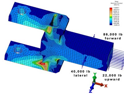
Finite Element Analysis (FEA) is a powerful tool that essentially divides a complex structure up into many small elements, where for each the stresses and deformations can be solved for using known equations of elasticity. Because the boundaries of each element in contact with another element must have equal and opposite forces and equal deflections, a large array of equations can be generated and solved by computer to determine the forces and deflections on all the elements. A critical issue is the constraints on the exterior elements that are meant to model the connection of the part to the world. For example, a cantilever beam has all the faces of elements at one end constrained to not have any deflections. But what about a simply supported beam?
 |
|---|
FEA configures a model for analysis using a complex system of points or nodes which are connected into a grid called a mesh. This mesh has defined properties or characteristics, such as material, structural properties, elasticity, etc.. The nodes are configured with particular density throughout the model dependant on the stress levels within a particular area. Areas that are know to relize elevated stress typically have a higher node density than those areas that will see little or no stress.
There are some types of elements, plates and shells that are two dimensional yet are assigned a thickness. These 2D elements can have an edge constrained to be simply supported (no linear displacement) or supported so there is no linear or angular displacement. Most design engineers creating new designs use a solid modeling system or Computer Aided Design (CAD) software, and the solid modeler is often parametrically linked directly to an FEA program. Herein lies the challenge, because some (not all) FEA programs take a solid model and break it up into solid elements, where their solid elements can only be constrained along a surface which causes a moment constraint (no linear or angular translations) to always be imposed. The moment constraint does not always capture the intent of the designer and can cause a structure’s stiffness to be greatly over predicted. Fortunately, as shown, some FEA programs do allow a solid’s edge to be displacement but not rotation constrained. If an FEA program does not allow the edge of a solid to be simply constrained, thin solid flexural elements can be added.
 |
|---|
General principles of FEA
The subdivision of a whole domain into simpler parts has several advantages:
- Accurate representation of complex geometry
- Inclusion of dissimilar material properties
- Easy representation of the total solution
- Capture of local effects.
A typical work out of the method involves (1) dividing the domain of the problem into a collection of subdomains, with each subdomain represented by a set of element equations to the original problem, followed by (2) systematically recombining all sets of element equations into a global system of equations for the final calculation. The global system of equations has known solution techniques, and can be calculated from the initial values of the original problem to obtain a numerical answer.
In the first step above, the element equations are simple equations that locally approximate the original complex equations to be studied, where the original equations are often partial differential equations (PDE). To explain the approximation in this process, FEM is commonly introduced as a special case of Galerkin method. The process, in mathematics language, is to construct an integral of the inner product of the residual and the weight functions and set the integral to zero. In simple terms, it is a procedure that minimizes the error of approximation by fitting trial functions into the PDE. The residual is the error caused by the trial functions, and the weight functions are polynomial approximation functions that project the residual. The process eliminates all the spatial derivatives from the PDE, thus approximating the PDE locally with
- a set of algebraic equations for steady state problems,
- a set of ordinary differential equations for transient problems.
These equation sets are the element equations. They are linear if the underlying PDE is linear, and vice versa. Algebraic equation sets that arise in the steady state problems are solved using numerical linear algebra methods, while ordinary differential equation sets that arise in the transient problems are solved by numerical integration using standard techniques such as Euler's method or the Runge-Kutta method.
In step (2) above, a global system of equations is generated from the element equations through a transformation of coordinates from the subdomains' local nodes to the domain's global nodes. This spatial transformation includes appropriate orientation adjustments as applied in relation to the reference coordinate system. The process is often carried out by FEM software using coordinate data generated from the subdomains.
FEM is best understood from its practical application, known as finite element analysis (FEA). FEA as applied in engineering is a computational tool for performing engineering analysis. It includes the use of mesh generation techniques for dividing a complex problem into small elements, as well as the use of software program coded with FEM algorithm. In applying FEA, the complex problem is usually a physical system with the underlying physics such as the Euler-Bernoulli beam equation, the heat equation, or the Navier-Stokes equations expressed in either PDE or integral equations, while the divided small elements of the complex problem represent different areas in the physical system.
FEA is a good choice for analyzing problems over complicated domains (like cars and oil pipelines), when the domain changes (as during a solid state reaction with a moving boundary), when the desired precision varies over the entire domain, or when the solution lacks smoothness. For instance, in a frontal crash simulation it is possible to increase prediction accuracy in "important" areas like the front of the car and reduce it in its rear (thus reducing cost of the simulation). Another example would be in numerical weather prediction, where it is more important to have accurate predictions over developing highly nonlinear phenomena (such as tropical cyclones in the atmosphere, or eddies in the ocean) rather than relatively calm areas.
Common FEA Applications
- Mechanical/Aerospace/Civil/Automotive Engineering
- Structural/Stress Analysis
- Static/Dynamic
- Linear/Nonlinear
- Fluid Flow
- Heat Transfer
- Electromagnetic Fields
- Soil Mechanics
- Acoustics
- Biomechanics
Link to this Webpage:
© Copyright 2000 -
2024, by Engineers Edge, LLC
www.engineersedge.com
All rights reserved
Disclaimer |
Feedback
Advertising
| Contact