Heat Rejection Waste Heat Thermodynamic Properties

Thermodynamics Directory | Heat Transfer Directory

Heat Rejection Waste Heat

Waste heat or heat rejection is by necessity produced both by machines that do work and in other processes that use energy , for example in a refrigerator warming the room air or a combustion engine releasing heat into the environment. The need for many systems to reject heat as a by-product of their operation is fundamental to the laws of thermodynamics . Waste heat has lower utility (or in thermodynamics lexicon a lower exergy or higher entropy ) than the original energy source. Sources of waste heat include all manner of human activities, natural systems, and all organisms.

Instead of being “wasted” by release into the ambient environment, sometimes waste heat (or cold) can be utilized by another process, or a portion of heat that would otherwise be wasted can be reused in the same process if make-up heat is added to the system (as with heat recovery ventilation in a building).

To understand why an efficiency of 73% is not possible we must analyze the Carnot cycle, thenc ompare the cycle using real and ideal components. We will do this by looking at the T-s diagrams of Carnot cycles using both real and ideal components. The energy added to a working fluid during the Carnot isothermal expansion is given by qs. Not all of this energy is available for use by the heat engine since a portion of it (qr) must be rejected to the environment.

This is given by:

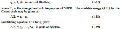
and is equal to the area of the shaded region labeled available energy in Figure 28 between the emperatures 1962 and 520R. From Figure 28 it can been seen that any cycle operating at a temperature of less than 1962R will be less efficient. Note that by developing materials capable of withstanding the stresses above 1962R, we could greatly add to the energy available for use by the plant cycle. From equation 1-37, one can see why the change in entropy can be defined as a measure of the energy unavailable to do work. If the temperature of the heat sink is known, then thec hange in entropy does correspond to a measure of the heat rejected by the engine

Figure 29 is a typical power cycle employed by a fossil fuel plant. The working fluid is water, which places certain restrictions on the cycle. If we wish to limit ourselves to operation at or below 2000 psia, it is readily apparent that constant heat addition at our maximum temperature of 1962R is not possible (Figure 29, 2 to 4). In reality, the nature of water and certain elements of the process controls require us to add heat in a constant pressure process instead (Figure 29, 1-2-3-4). Because of this, the average temperature at which we are adding heat is far below the maximum allowable material temperature. As can be seen, the actual available energy (area under the 1-2-3-4 curve, Figure 29) is less than half of what is available from the ideal Carnot cycle (area under 1-2-4 curve, Figure 29) operating between the same two temperatures. Typical thermal efficiencies for fossil plants are on the order of 40% while nuclear plants have efficiencies of the order of 31%. Note that these numbers are less than 1/2 of the maximum thermal efficiency of the ideal Carnot cycle calculated earlier. Figure 30 shows a proposed Carnot steam cycle superimposed on a T-s diagram. As shown, it has several problems which make it undesirable as a practical power cycle. First a great deal of pump work is required to compress a two phase mixture of water and steam from point 1 to the saturated liquid state at point 2 . Second, this same is entropic compression will probably result in some pump cavitation in the feed system. Finally, a condenser designed to produce a two-phase mixture at the outlet (point1) would pose technical problems.

Early thermodynamic developments were centered around improving the performance of contemporary steam engines. It was desirable to construct a cycle that was as close to being reversible as possible and would better lend itself to the characteristics of steam and process control than the Carnot cycle did. Towards this end, the Rankine cycle was developed. The main feature of the Rankine cycle, shown in Figure 31, is that it confines the isentropic compression process to the liquid phase only (Figure 31 points 1 to 2). This minimizes the amount of work required to attain operating pressures and avoids themechanical problems associated with pumping at wo-phase mixture. The compression process shown in figure 31 between points 1 and 2 is greatly exaggerated*. In reality, a temperature rise of only 1 F occurs in compressing water from 14.7 psig at a saturation temperature of 212F to 1000 psig.

In a Rankine cycle available and unavailable energy on a T-s diagram, like a T-s diagram of a Carnot cycle, is represented by the areas under the curves. The larger the unavailable energy, the less efficient the cycle.

From the T-s diagram (Figure 32) it can also be seen that if an ideal component, in this case the turbine, is replaced with an on-ideal component, the efficiency of the cycle will be reduced. This is due to the fact that then on-ideal turbine incurs an increase in entropy which increases the are a under the T-s curve for the cycle. But the increase in the area of available energy (3-2-3, Figure 32) is less than the increase in area for unavailable energy (a-3-3-b, Figure 32).

The same loss of cycle efficiency can be seen when two Rankine cyclesare compared (see Figure 33). Using this type of comparison, the amount of rejected energy to available energy of one cycle can be compared to another cycle to determine which cycle is the most efficient, i.e. has the least amount of unavailable energy. An h-s diagram canal so be used to compare systems and help determine their efficiencies. Like the T-s diagram, the h-s diagram will show (Figure 34) that substituting non-ideal components in place of ideal components in a cycle, will result in the reduction in the cycles efficiency. This is because a change in enthalpy (h) always occurs when work is done or heat is added or removed in an actual cycle (non-ideal). This deviation from an ideal constant enthalpy (vertical line on the diagram) allows the inefficiencies of the cycle to be easily seen on a h-s diagram.