Analysis Reciprocating Engine Connecting Rods
Strength of Materials and Analysis
Tension and Compression Analysis in Reciprocating Engine Connecting Rods
A Failure Analysis
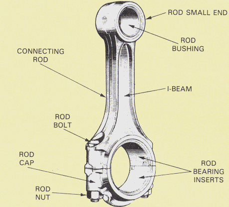
Contributed by: Jessie Nichols
Original work by: Luke Schreier
INTRODUCTION
In order to understand the true impact the automobile has had on our society, we would have to go back in time over one hundred years. A time without the simplicity of hopping into a vehicle to take us anywhere we want to go is almost unfathomable to many Americans. But for the early automotive engineers, the tremendous advancements in automotive technology would be even more surprising.
In the last 50 years, cars have learned to think, adjust, and even protect. But this is just the tip of the iceberg. High performance is now the catch phrase. The vast majority of people want a vehicle that will get them from point A to point B as easily as possible, but also put a little smile on their faces. Often times, the smile is created by a quick punch of the accelerator and accompanied by a feeling of immense power and control. The auto manufacturers are well aware of this, and to achieve it, they design faster, lighter, and more efficient engines to do the job. But exactly what happens inside an engine, and what are the risks involved in designing the strongest engine on the block?
In this project, one component of an engine in particular, the connecting rod, will be analyzed. Being one of the most integral parts in an engine’s design, the connecting rod must be able to withstand tremendous loads and transmit a great deal of power. It is no surprise that a failure in a connecting rod can be one of the most costly and damaging failures in an engine. But simply saying that isn’t enough to fully understand the dynamics of the situation.
Throughout the course of this project, an idealized model of a connecting rod, piston, and flywheel will be modeled and analyzed. It will become apparent exactly why these parts are so important to the operation of an automobile, and furthermore how prone to failure they can be. However, before too much more is said on the engineering details, a little background information is necessary.
FUNDAMENTALS
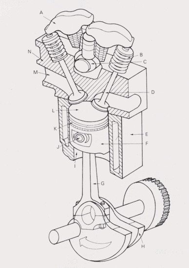 Below is a picture of the fundamental parts of an
engine. Surface "L" is where combustion occurs, air enters through "M", and "H"
is the shaft through which power is accumulated and delivered out of the engine.
The combustion occurs against the top surface of the piston (F) and pushes the
connecting rod (G) downward, causing the shaft to move in a circular motion. So,
it is easy to see that the connecting rod harnesses all of the power produced in
combustion and converts it into something useful, in this case a spinning
shaft.
ASSUMPTIONS AND FREE-BODY DIAGRAMS
Now that we are all on the same page, the assumptions for this project can be discussed. First of all, it is necessary to point out that the actual dynamics of such a system are tremendous, and to model all of them in one project would be quite a task. So, to simplify, this project will neglect momentum and gravity. Only one connecting rod-piston assembly will be considered. The crankshaft, while in actuality having a very functional mass distribution, will be considered simply a circle (or if it is easier to visualize, a flywheel). In effect, many of the same calculations could be performed on a more sophisticated system, but this will suffice for the time being.
Here is what we start with:
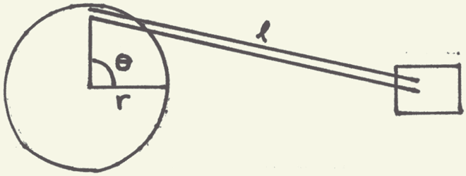
From an understanding of statics, we can represent the connecting rod of length "l" by a two-force member (this requires a few more assumptions, but for purposes of this project, it is acceptable). Given this, we can split this system into two free-body diagrams:

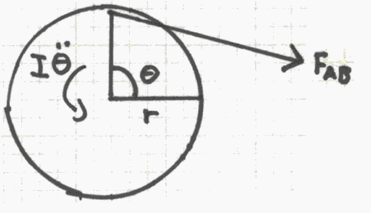
EQUATIONS
From these free-body diagrams, we can apply Newton’s Second Law (F=ma) to write some equations. In particular, we are interested in summing forces in the "x" direction (horizontal), and summing the moments about the center of the flywheel. Doing so, we acquire these equations:
S Mo = -FAB cos (F ) * rsin (Q ) – FAB sin (F ) * rcos(Q ) = I * d2Q /dt2 (CCW positive)
S Fx = -FAB cos (F ) – P = m * d2x/dt2 (® positive)
We can simplify the moment equation, employing the use of the double-angle trigonometric formula:
sin (F + Q ) = cos (F ) * sin (Q ) + sin (F ) * cos (Q )
Therefore,
-FAB * r sin (F + Q ) = I * d2Q /dt2
Now, if we solve the force equation for –FAB,
-FAB = (m * d2x/dt2 + P)/(cos (F ))
We can substitute this equation into our moment equation, giving us:
(m * d2x/dt2 + P)/cos (F ) * r sin (F + Q ) = I * d2 /dt2
This will be our main equation of rotation.
At this point, we are working our way towards acquiring a representation of Q , in order to eventually find FAB. But looking at these equations, we can see that there are many different variables to work with, including a few derivatives. In order to help simplify them a little more, it is important to notice a few relations. For instance, we can apply the law of sines to this triangle, found between the flywheel and piston:
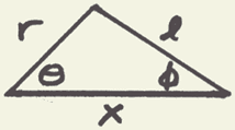
sin (Q )/l = sin (F )/r 2
This takes care of the two angles. Next, we must find an equation for x, the distance from the center of the flywheel to the bottom of the piston. This can be found using trigonometry:

x = l cos (F ) + r cos (Q )
Unfortunately, we are not actually dealing with x in this problem, but rather d2x/dt2. Therefore, we will have to take two derivatives of x:
dx/dt = -l sin (F ) * dF /dt – r sin (Q ) * dQ /dt
d2x/dt2 = -l cos (F )*(dF /dt)2 – l sin (F )*(d2F /dt2) – r cos (Q )*(dQ /dt)2 –
r sin (Q )* d2Q /dt2
With this value for d2x/dt2, we can substitute back into our main equation. However, once again we have introduced a few more items into this scenario, in particular the first and second derivatives or Q and F . Given these terms, we will once again have to find equations that relate them to things we already know or can find.
Because this is a long process, I will explain what is happening beforehand and then simply show the equations. We have our equation relating Q and F that was derived from the law of sines. From this, we can take a few more derivatives to find equations for dF /dt and d2F /dt2. It is not necessary to find the relation of the derivatives of Q because they will be shown in the final integrations.
F = sin-1((r sin (Q ))/l)
dF /dt = r sin (Q ) * dQ /dt
l cos (F )
d2F /dt2 = -r cos (Q ) * (dQ /dt)2 + r sin (Q ) * d2Q /dt2 + sin (F ) * (dF /dt)2
l cos (F ) l cos (F ) cos (F )
PRESSURE IN A FOUR-STROKE ENGINE
Up to this point, the variable P has gone unmentioned. The pressure in the cylinder (P) is not an easy thing to model for a situation like this, yet it is one of the most important factors in the final analysis. To be able to explain how P fluctuates, it is once again necessary to give a little background on a four-stroke engine.
A four-stroke engine is the most common type used in automobiles. The four strokes are intake, compression, power, and exhaust. Each stroke requires approximately 180 degrees of crankshaft (or flywheel) rotation, so the complete cycle would take 720 degrees. Each stroke plays a very important role in the combustion process, and each has a different pressure surrounding it.
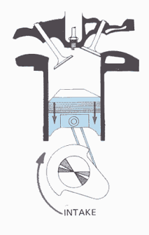 In the intake cycle, as the picture shows, the piston is
moving downward while one of the valves is open. This creates a vacuum, and an
air-fuel mixture is sucked into the chamber. This would be cause for very little
pressure on the piston, so P is small.
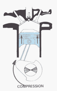 Moving on to compression, we can see that both valves are
closed, and the piston is moving upward. This creates a much larger amount of
pressure on the piston, so we would have a different representation of P in our
equation for this stroke.
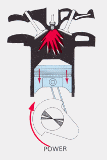 The next stroke is the big one: power. This is where the
compressed air-fuel mixture is ignited with a spark, causing a tremendous jump
in pressure as the fuel burns. The pressure seems to "spike", so the most cause
for concern occurs here. (This is also the area in which the dangers of engine
knock or pre-detonation can occur, causing an even larger spike.)
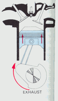 Finally, we have the exhaust stroke. In this stroke, the
exhaust valve is open, once again creating a chamber of low pressure. So, as the
piston moves back upwards, it forces all the air out of the chamber. The
pressure in this region is therefore considered very low.
So, given the understanding of how a four-stroke engine works, we must now model the variable pressure for all 720 degrees (or 12.57 radians). Creating a piecewise-defined function does this. However, we still need to find some basic values for the pressure, and for the purposes of this project, a particular graphical representation was chosen:
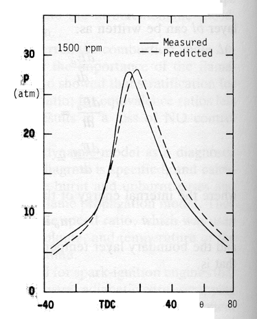
In order to make this graph work, we assume all points are linearly connected. In other words, three pressures were selected (5, 10, and 30 atm), and it was assumed that the pressure increased linearly between them. With this assumption, the piecewise-defined function became (angles in radians):
P = 10 +200*Q 0 < Q < .1
30 .1 £ Q < .35
30 + (20-57.14*Q ) .35 £ Q < .7
10 + (5-7.14*Q ) .7 £ Q < 1.4
5 1.4 £ Q < 11.87
5 + 7.14*Q 11.87 £ Q < 12.57
INTEGRATION AND DATA ANALYSIS
Now that we have everything represented in one way or another, it becomes necessary to focus our attention on finding Q . Because such a complicated equation cannot be solved analytically, a numerical method needs to be used. In this particular case, given its complexity, the Euler method of integration was chosen.
 In order to perform all of the calculations, a program was
written in Fortran. Essentially, it asked for the mass, radius, and length from
the user, as well as the starting values of Q , dQ /dt, and d2Q
/dt2 and the time step value, while producing the values of
Q and the actual force in the connecting rod,
FAB. In order to analyze the data over a period of time, the Q and FAB values were sent to a file, which was
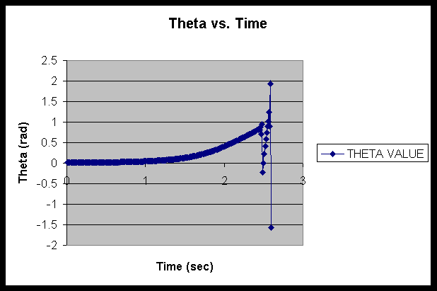
read by Microsoft Excel and graphed over time. The two graphs, Q vs. time and FAB vs. time, are displayed below.
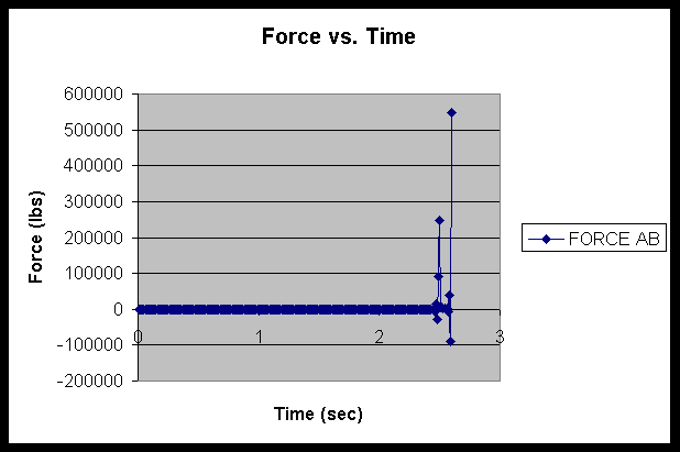
Note: For purposes of this project, the following substitutions were made: the length was set equal to 6.7 in, radius of the flywheel was 4.33 in, the radius of the piston was 2.31 in, and the mass of the piston was 3 lbs.
DATA IMPLICATIONS
It appears from looking at the graphs that a mistake must have been made. It would take far less time for a flywheel to rotate than the 10-15 seconds that could be inferred from the graph of theta. In addition to that, we would also assume theta to be constantly increasing as opposed to the rapid fluctuations it experiences here. Unfortunately, it is very difficult to say what is causing this error. There is always the chance of mathematical errors occurring, but it could also have been due to the fact that the system started out from rest. In actuality, a starter would give the flywheel an initial turn or two to get things moving, letting combustion eventually take over. However, that becomes very difficult to model in this case.
Generally, we would assume that because our graph of theta is incorrect, the graph of force is probably as incorrect. However, looking at it, we see that there are certain areas where the force is much greater. This is definitely expected, but probably not to the degree that it shows up. But, for the sake of discussion, let us just assume that the high value of around 550,000 lbs that shows up on our graph is actually correct. Making that assumption, we can do some calculations and relate this data to the Mechanics of Materials.
First of all, to find the stress on the connecting rod, we use the formula:
s = P/A (s = stress, P = force acting on rod, A = cross-sectional area)
If we assume a connecting rod thickness of approximately .5 in and a width of 1.25 in, we would calculate a cross-sectional area of .625 in2. Therefore, plugging in our values of P=550,000 lbs and A=.625 in2, we would get a stress of 880,000 pounds per in2.
Now what does this value mean to us? Is this a lot of stress to place on a material? Well, let’s assume that the two most likely materials to be used in a connecting rods are steel and aluminum. This is actually a pretty good assumption, since the vast majority of automobiles contain steel or aluminum rods.
STRESS-STRAIN DIAGRAMS
To understand the strength of each material in a situation like this, we need to understand a stress-strain diagram (pictured below). Each material behaves in a similar manner when placed under a load. There is a period of elastic deformation, in which the material is stretched, but it returns to its original size when unloaded. The point at which it fails to return to the original specifications is called the yield stress. Now, in an automobile, we would probably have to assume that this yield stress would be passed at some point, so most connecting rods come out of engines a different size than when they were installed.
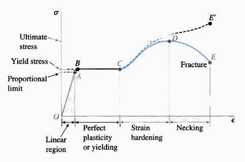
After the yield stress, another stress point can be reached called the ultimate stress point. At this point, a material has essentially reached the point of no return. Failure is imminent, and even a decreased amount of stress can cause fracture. So, naturally, this is what we concern ourselves with.
For the type of steel that a connecting rod would likely be created with, the ultimate tensile strength would be about 80 to 180 thousand pounds per in2. If aluminum were used, the ultimate tensile strength would be closer to 70 thousand pounds per in2. So, you can see that our connecting rod, under a stress of 880 thousand psi, would be in serious trouble. Failure would almost definitely occur, even if incredibly high strength steel were used.
REAL-WORLD RELATION
It is in calculations like these that automotive engineers are able to predict exactly what materials and specifications can be used in a high-performance engine. While the data that was produced in this project appeared to be flawed, data similar to it can be produced for each type of engine produced. Without such knowledge, there would be a lot of guessing, and with guessing usually comes catastrophe.
ANOTHER SOURCE ON THE MATTER
In an article appearing in the newsstand magazine "Engines", Jim McFarland writes a nice article describing the most common types of failure in connecting rods. Much of what he writes about is similar to the concepts in this project, but he throws in a few more interesting comments.
For the most part, the type of fracture considered in this project occurred in the center of the rod. McFarland also touches on failure at the connecting rod bolts. These bolts attach the rods to the crankshaft journals, and consequently, they are placed under just as much strain as the rod itself. He states that they are often made to withstand stresses in excess of 250,000 psi. (Which, by the way, is an awful long was from 880,000 psi, further showing how inaccurate our data appears to be.)
As I alluded to earlier, abnormal combustion is also a serious problem for connecting rods. McFarland notes that under detonation conditions, the pressure from combustion can be almost double what it normally might be. Understanding this, we can see just how susceptible a connecting rod could be to using the wrong gasoline. (Improper octane ratings are often a causing of pinging or knocking in an engine.)
CONCLUDING NOTES
If anything, this project should have conveyed a sense of just how erratically an engine can operate, even under normal conditions. It is this lack of continuity that can create major problems on parts like connecting rods. Hence, designers and engineers are forced to choose materials that are strong enough to withstand such powerful forces, while maintaining a low cost and lightweight product.
Despite the fact the data in this project appeared incorrect in the final analysis, the thought process behind it was very typical of what must be done to analyze a complicated system. If a more accurate analysis was necessary, factors like cylinder friction, momentum, and dozens of other variables could have been taken into account. But, given the assumptions that were made and the data acquired, this project still provided an interesting look at what happens inside an engine and what limitations each engine has placed upon it.
REFERENCES
- Duffy, James E. Modern Automotive Technology. 1994, Goodheart-Wilcox Company.
- McFarland, Jim. "Connecting Rod Basics." Engines. March, 1999. Peterson Publishing Company.
- Ramos, J.I. Internal Combusion Engine Modeling. 1989, Hemisphere Publishing.
- Gere and Timoshenko. Mechanics of Materials: Fourth Edition. 1997, PWS Publishing Company.
- Beer and Johnston. Vector Mechanics for Engineers: Dynamics. 1997, WCB/McGraw-Hill.